Using geom_ribbon() to visualize a corridor for your data
Contents
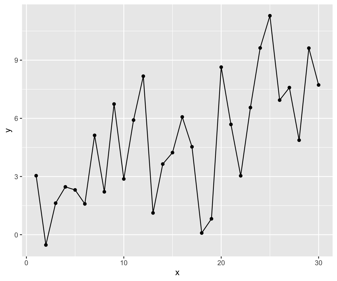
Let’s say you have some data like this
|
|
So let’s plot it using ggplot:
|
|
Plotting an aim-corridor
If this is something like your revenue, pageviews or something like that you may ask: “Is this good or is this bad?”
So chances are good you have an aim for this data like this one here and merge it with your data
|
|
Now we can use ggplot’s geom_ribbon to plot this corridor:
|
|
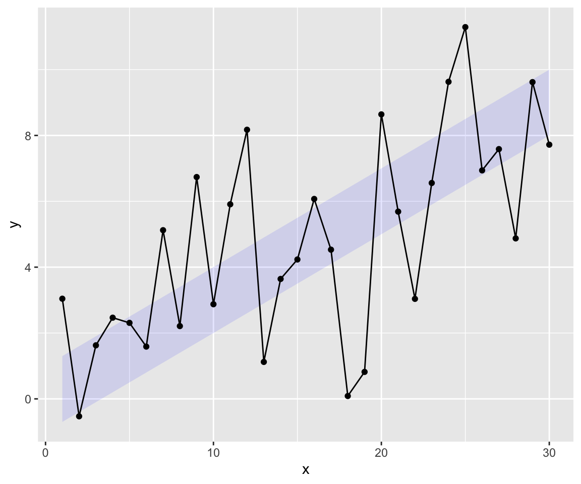
The result looks better. But there is even an enhancement possible.
Fully colour-coding the area above and below the corridor
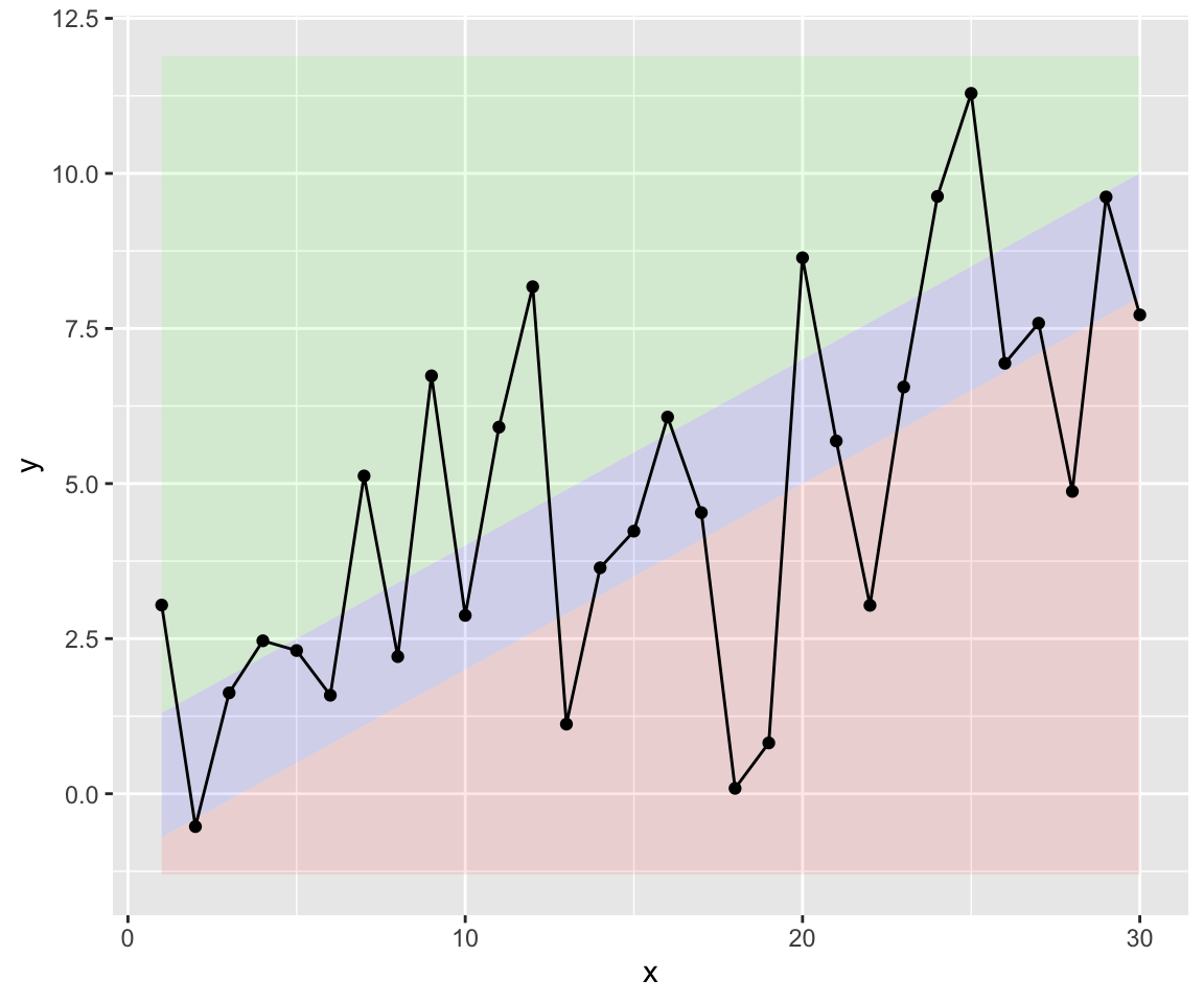
But now the question is if it’s better to be above or below the corridor? Think about cost per customer. Than below the corridor is better. But if the data is revenue per customer above the corridor would be better.
So let’s colour-code the areas below and above the corridor.
Therefor we need to now the boundaries of the actual plot. We use the function ggplot_build to get the meta-info of the plot and plot it again:
I’ve updated this snippet because ggplot2 2.2.x now uses panel_ranges instead of ranges.
I’ve updated this snippet again because ggplot2 3.3.x now uses panel_params instead of panel_ranges.
|
|
Next steps
I would like encapsulate the whole process of generating the corridor and the areas above and below into a new geom. So I would like to write an extension to ggplot as mentioned in the documentation of ggplot2. But I haven’t done that yet.