Last Thursday I watched Wolfgang Viechtbauer’s stream
on Twitch. Wolfgang spoke about linear regression.
(If you’re interested in the results: Wolfgang lists the R-code he wrote during
the stream at https://www.wvbauer.com/doku.php/live_streams.)
During the stream we had an example with one categorical and one numeric predictor
and we built a model with interaction between these two predictors.
So the result is a straight line for each value of the categorival group.
The question was if it makes a difference if you build a simple linear model for
each group.
So let’s look at it.
Example
Let’s start and build some sample data:
 1
 2
 3
 4
 5
 6
 7
 8
 9
10
11
12
13
14
15
16
17
18
19
20
21
22
23
|
options(tidyverse.quiet = TRUE)
library(tidyverse)
parameters <- tribble(
  ~class_name, ~intercept, ~slope, ~sd,
  "A", 5, 0.5, 5,
  "B", 6, -0.5, 5,
  "C", 7, 1, 5,
)

generate_class <- function(n, class_name, intercept, slope, sd) {
  start <-  0
  end   <- 10
  values <- tibble(
    class_name = rep(class_name, times = n),
    x          = runif(n, start, end),
    y          = intercept + x * slope + rnorm(n, sd)
  )

  return(values)
}

set.seed(42)
data <- pmap_dfr(parameters %>% mutate(n = 20), generate_class)
|
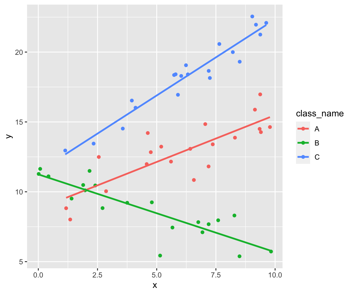
So we get three clouds of points. Each cloud follows its own line.
1
2
3
4
|
data %>%
  ggplot(aes(x, y, color = class_name)) +
  geom_point() +
  stat_smooth(formula = y ~ x, method = lm, se = FALSE)
|
Build one linear model
We’re building the model without an intercept by using 0 + as start of the
formula so we get the intercept for each group directly (without building the
sum of the reference group and the other groups.)
1
2
|
model_complete <- lm(y ~ 0 + class_name + class_name:x, data = data)
summary(model_complete)
|
 1
 2
 3
 4
 5
 6
 7
 8
 9
10
11
12
13
14
15
16
17
18
19
20
21
22
|
##
## Call:
## lm(formula = y ~ 0 + class_name + class_name:x, data = data)
##
## Residuals:
##      Min       1Q   Median       3Q      Max
## -2.94880 -0.65484  0.06566  0.66447  2.32326
##
## Coefficients:
##               Estimate Std. Error t value Pr(>|t|)
## class_nameA    8.78346    0.60220  14.586  < 2e-16 ***
## class_nameB   11.24628    0.42291  26.592  < 2e-16 ***
## class_nameC   11.43872    0.69364  16.491  < 2e-16 ***
## class_nameA:x  0.67056    0.09012   7.441 7.93e-10 ***
## class_nameB:x -0.55649    0.07967  -6.985 4.35e-09 ***
## class_nameC:x  1.09090    0.10240  10.653 6.95e-15 ***
## ---
## Signif. codes:  0 '***' 0.001 '**' 0.01 '*' 0.05 '.' 0.1 ' ' 1
##
## Residual standard error: 1.071 on 54 degrees of freedom
## Multiple R-squared:  0.9948,	Adjusted R-squared:  0.9942
## F-statistic:  1727 on 6 and 54 DF,  p-value: < 2.2e-16
|
Build three different models
Now build a linear model for each group.
1
2
3
4
5
|
model_split <- data %>%
  group_by(class_name) %>%
  group_map(~ coef(summary(lm(y ~ x, data = .x))))

model_split
|
 1
 2
 3
 4
 5
 6
 7
 8
 9
10
11
12
13
14
|
## [[1]]
##              Estimate Std. Error   t value     Pr(>|t|)
## (Intercept) 8.7834572  0.7482108 11.739282 7.181449e-10
## x           0.6705587  0.1119703  5.988718 1.153349e-05
##
## [[2]]
##               Estimate Std. Error   t value     Pr(>|t|)
## (Intercept) 11.2462761 0.40929811 27.476980 3.773904e-16
## x           -0.5564857 0.07710095 -7.217624 1.027562e-06
##
## [[3]]
##              Estimate Std. Error  t value     Pr(>|t|)
## (Intercept) 11.438716  0.5000135 22.87681 9.354783e-15
## x            1.090904  0.0738192 14.77805 1.653770e-11
|
Comparison
As you can see the coefficients are the same but the standard error of the
coefficients are different.
“What’s the reason?” I was asking myself.
Simple example
So I began to look at a simpler example:
 1
 2
 3
 4
 5
 6
 7
 8
 9
10
11
|
data <- tribble(
  ~class_name,  ~x, ~y,
  "A", 0, 1,
  "A", 10, 11,
  "A", 10, 21,
  "B", 0, 0,
  "B", 10, 0,
  "B", 10, 5,
)

data
|
1
2
3
4
5
6
7
8
9
|
## # A tibble: 6 x 3
##   class_name     x     y
##   <chr>      <dbl> <dbl>
## 1 A              0     1
## 2 A             10    11
## 3 A             10    21
## 4 B              0     0
## 5 B             10     0
## 6 B             10     5
|
1
2
3
4
|
data %>%
  ggplot(aes(x, y, color = class_name)) +
  geom_point() +
  stat_smooth(formula = y ~ x, method = lm, se = FALSE)
|
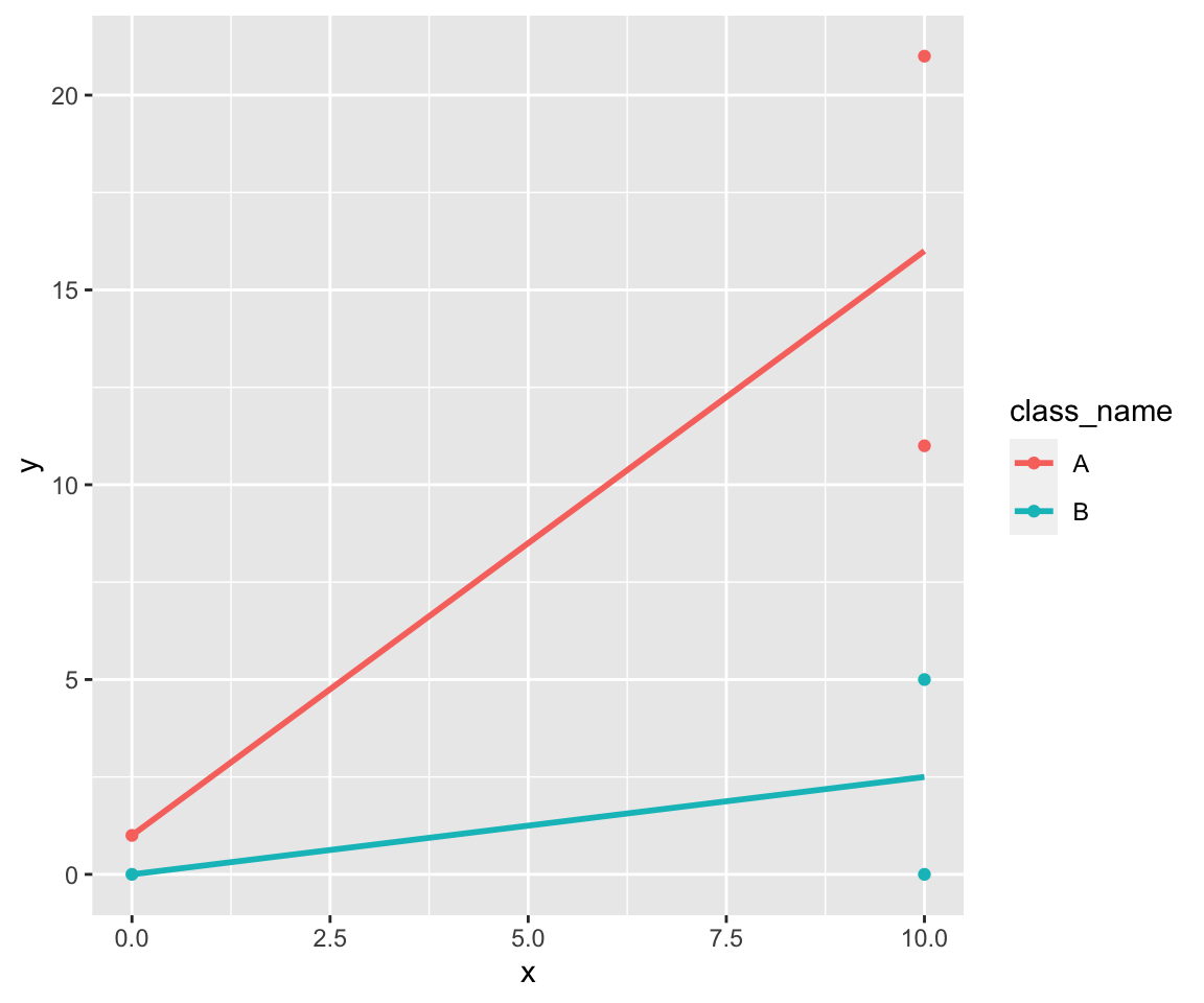
So we’ve only two groups. The linear model is simple:
1
|
lm(y ~ class_name * x, data) %>% summary()
|
 1
 2
 3
 4
 5
 6
 7
 8
 9
10
11
12
13
14
15
16
17
18
|
##
## Call:
## lm(formula = y ~ class_name * x, data = data)
##
## Residuals:
##          1          2          3          4          5          6
## -4.441e-16 -5.000e+00  5.000e+00  1.648e-15 -2.500e+00  2.500e+00
##
## Coefficients:
##               Estimate Std. Error t value Pr(>|t|)
## (Intercept)     1.0000     5.5902   0.179    0.875
## class_nameB    -1.0000     7.9057  -0.126    0.911
## x               1.5000     0.6847   2.191    0.160
## class_nameB:x  -1.2500     0.9682  -1.291    0.326
##
## Residual standard error: 5.59 on 2 degrees of freedom
## Multiple R-squared:  0.8201,	Adjusted R-squared:  0.5501
## F-statistic: 3.038 on 3 and 2 DF,  p-value: 0.2574
|
Step by Step computation
But how can we compute the linear model step by step?
The data
First let’s split the data into $ y $ and $ X $:
 1
 2
 3
 4
 5
 6
 7
 8
 9
10
11
12
|
y <- data %>% pull(y)
X <- data %>%
  mutate(
    x0 = 1,
    x1 = class_name != "A",
    x2 = x,
    x3 = x1*x
    ) %>%
  select(x0, x1, x2, x3) %>%
  as.matrix()

X
|
1
2
3
4
5
6
7
|
##      x0 x1 x2 x3
## [1,]  1  0  0  0
## [2,]  1  0 10  0
## [3,]  1  0 10  0
## [4,]  1  1  0  0
## [5,]  1  1 10 10
## [6,]  1  1 10 10
|
So $ y $ contains the values of the dependent variable. $ X $ is a matrix with
$ 1 $ in the first column called $ x_0 $. $ x_1 .. x_3 $ are the predictors.
$ x_3 $ is the interaction between $ x_1 $ and $ x_2 $.
The model
Now we can write our model as:
$$
y = X \beta + \epsilon
$$
We’re searching for $ b $ so that $ \hat{y} = X b $ is the
prediction which minimizes the sum of the squared residuals.
We get $ b $ as
$$
b = (X^t X)^{-1} X^t y
$$
So let’s compute it: (solve computes the inverse of a matrix)
1
2
3
4
|
Xt <- t(X)

b <- solve(Xt %*% X) %*% Xt %*% y
round(b, 3)
|
1
2
3
4
5
|
##     [,1]
## x0  1.00
## x1 -1.00
## x2  1.50
## x3 -1.25
|
Standard Errors of the coefficients
Now we’re looking at the standard errors of the coefficients:
We can compute them by
$$
Cov(b) = \sigma^2 (X^t X)^{-1}
$$
A predictior for $ \sigma^2 $ is the mean squared error:
$$
s^2 = \frac{\sum{(y_i - \hat{y})^2}}{df}
$$
In our case the degrees of freedom are $ df = n - 4 $.
1
2
3
4
|
yh <- X %*% b
df <- length(y) - 4
MSE <- sum((y - yh)**2) / df
MSE
|
So the standard errors of the coefficients are the main diagonal of this matrix:
1
|
(solve(Xt %*% X) * MSE) %>% sqrt()
|
1
|
## Warning in sqrt(.): NaNs produced
|
1
2
3
4
5
|
##          x0       x1        x2        x3
## x0 5.590170      NaN       NaN 1.7677670
## x1      NaN 7.905694 1.7677670       NaN
## x2      NaN 1.767767 0.6846532       NaN
## x3 1.767767      NaN       NaN 0.9682458
|
These are the same as computed by lm:
1
|
lm(y ~ class_name * x, data) %>% summary()
|
 1
 2
 3
 4
 5
 6
 7
 8
 9
10
11
12
13
14
15
16
17
18
|
##
## Call:
## lm(formula = y ~ class_name * x, data = data)
##
## Residuals:
##          1          2          3          4          5          6
## -4.441e-16 -5.000e+00  5.000e+00  1.648e-15 -2.500e+00  2.500e+00
##
## Coefficients:
##               Estimate Std. Error t value Pr(>|t|)
## (Intercept)     1.0000     5.5902   0.179    0.875
## class_nameB    -1.0000     7.9057  -0.126    0.911
## x               1.5000     0.6847   2.191    0.160
## class_nameB:x  -1.2500     0.9682  -1.291    0.326
##
## Residual standard error: 5.59 on 2 degrees of freedom
## Multiple R-squared:  0.8201,	Adjusted R-squared:  0.5501
## F-statistic: 3.038 on 3 and 2 DF,  p-value: 0.2574
|
As you can see the covariance matrix isn’t diagnal. Points from “the other group”
also effect the standard error.
So the errors are different to the errors of two independent models:
1
2
3
|
data %>%
  group_by(class_name) %>%
  group_map(~ coef(summary(lm(y ~ x, data = .x))))
|
1
2
3
4
5
6
7
8
9
|
## [[1]]
##             Estimate Std. Error   t value  Pr(>|t|)
## (Intercept)      1.0  7.0710678 0.1414214 0.9105615
## x                1.5  0.8660254 1.7320508 0.3333333
##
## [[2]]
##                Estimate Std. Error      t value  Pr(>|t|)
## (Intercept) 2.56395e-16  3.5355339 7.251946e-17 1.0000000
## x           2.50000e-01  0.4330127 5.773503e-01 0.6666667
|
Separate Models
For completeness let’s check the manual way for one single model here:
 1
 2
 3
 4
 5
 6
 7
 8
 9
10
11
12
13
14
15
|
data_single <-data %>%
  filter(class_name == "A")

y <- data_single %>% pull(y)
X <- data_single %>%
  mutate(
    x0 = 1,
    x1 = class_name != "A",
    x2 = x,
    x3 = x1*x
    ) %>%
  select(x0, x2) %>%
  as.matrix()

X
|
1
2
3
4
|
##      x0 x2
## [1,]  1  0
## [2,]  1 10
## [3,]  1 10
|
1
2
3
4
|
Xt <- t(X)

b <- solve(Xt %*% X) %*% Xt %*% y
round(b, 3)
|
1
2
3
|
##    [,1]
## x0  1.0
## x2  1.5
|
1
2
3
4
|
yh <- X %*% b
df <- length(y) - 2
MSE <- sum((y - yh)**2) / df
MSE
|
1
|
(solve(Xt %*% X) * MSE) %>% sqrt()
|
1
|
## Warning in sqrt(.): NaNs produced
|
1
2
3
|
##          x0        x2
## x0 7.071068       NaN
## x2      NaN 0.8660254
|
Further reading
For more information about multilinear regression look at